


from sklearn.cluster import KMeans

scaled_df, X_features
Out:
(      Freq_scaled  SaleAmount_scaled  ElapsedDays_scaled
 0       -2.438202           3.707716            1.409894
 1        1.188986           1.414903           -2.146498
 2       -0.211465           0.720024            0.383971
 3        0.461819           0.702287           -0.574674
 4       -0.673554          -0.614514            1.374758
 ...           ...                ...                 ...
 4333    -1.069075          -1.102093            1.298690
 4334    -1.324833          -1.735717            0.999081
 4335    -0.934910          -1.113332           -1.178605
 4336     2.291307           0.822812           -1.662552
 4337     0.428581           0.737526           -0.004422

 [4338 rows x 3 columns],
 array([[-2.43820181,  3.7077163 ,  1.40989446],
        [ 1.18898578,  1.41490344, -2.14649825],
        [-0.21146474,  0.72002428,  0.38397128],
        ...,
        [-0.9349095 , -1.11333158, -1.17860486],
        [ 2.29130702,  0.82281217, -1.66255156],
        [ 0.42858139,  0.73752572, -0.00442205]]))
We selected and scaled three features as the basis for our clustering. In other words, the features that the algorithm considers when comparing the values of two data points. We will use the X_features as an input to the KMeans algorithm. The algorithm will then form clusters based on these three features:
Customer 1: 'Freq' of 10, 'SaleAmount' of $500, 'ElapsedDays' of 30.
Customer 2: 'Freq' of 8, 'SaleAmount' of $450, 'ElapsedDays' of 35.
The K-means algorithm might consider these two customers to be similar because the values of their features are relatively close. The features of both customers are within the same range.
On the other hand, consider a third customer:
- Customer 3: 'Freq' of 2, 'SaleAmount' of $50, 'ElapsedDays' of 180.
Customer 3 is quite different from Customers 1 and 2, based on their frequency of purchase, the total amount they spent, and the elapsed days since their first purchase. The K-means algorithm would likely place this customer in a different cluster from the first two.
The K-means algorithm requires the number of clusters, denoted by k, as an input. K refers how many of these groups we want the algorithm to create. If we don't provide the number of these groups, the algorithm randomly selects k data points from our dataset to serve as the initial centroids. This is a parameter we set before running the algorithm, and choosing the right value can have a big impact on the results.
Let's proceed from the part where we choose an appropriate number of clusters using the Elbow method, then we fit the K-means model to the data to assign each data point to one of the clusters.
# Fitting the KMeans model for a range of number of clusters
# The WCSS for each number of clusters (from 1 to 10) is computed and stored in the list `wcss`.
wcss = []
for i in range(1, 11):
    kmeans = KMeans(n_clusters=i, init='k-means++', max_iter=300, n_init=10, random_state=0)
    kmeans.fit(X_features)
    wcss.append(kmeans.inertia_)

# Plotting the results onto a line graph to observe the 'elbow'
plt.plot(range(1, 11), wcss)
plt.title('Elbow Method')
plt.xlabel('Number of clusters')
plt.ylabel('WCSS')
plt.show()
Out:
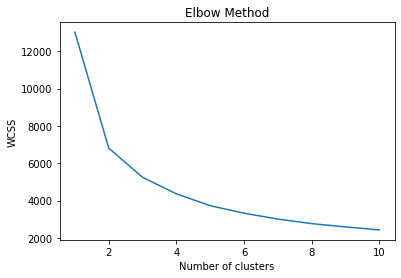
Determining the optimal number of clusters by using the Elbow method involves fitting the model with a range of k values and plotting the corresponding inertia (the within-cluster sum-of-squares), a measure of how internally coherent the clusters are. WCSS quantifies how far each data point in a cluster is from the centroid of that cluster. The smaller the inertia value, the closer all the points in a cluster are, which means the better our clustering has performed.
The Elbow method is a technique for choosing a good value for K. Here's how it works:
For each number of clusters in our range (e.g., 1 to 10), we perform the K-means clustering and calculate the total inertia (or WCSS).
We then plot these inertia values on a graph, with the number of clusters on the x-axis and the inertia value on the y-axis.
This plot looks a bit like an arm, with a steep decline that flattens out at some point, forming an "elbow".
You're looking for a point where the change in WCSS begins to level off (the "elbow"), which often indicates a good number of clusters to use. The idea is that the inertia decreases as we increase the number of clusters, but at some point, the decrease becomes much less pronounced (in this case, around 3). The value of this point represents a balance between minimizing inertia (having well-separated clusters) and not having too many clusters.
Once we've determined the optimal number of clusters based on WCSS, we can run the K-Means algorithm with that number of clusters and assign the labels to the data frame.
# we'll assume that we chose 3 as the optimal number of clusters
num_clusters = 3

# initialize KMeans with the chosen number of clusters
kmeans = KMeans(n_clusters=num_clusters, init='k-means++', max_iter=300, n_init=10, random_state=0)

# fit the model to the data
labels = kmeans.fit_predict(X_features)

# Add the cluster labels for each data point to the dataframe
customer_df['ClusterLabel'] = labels
In this block of code, we create a new instance of the
KMeansclass, telling it to findnum_clustersclusters in our data and it randomly initializes the centroids by default.The KMeans algorithm will run 10 separate times (as specified by
n_init=10), each with a different initial configuration of centroids. Each of these 10 runs will have up to 300 iterations (as specified bymax_iter=300).During each iteration, the algorithm updates the cluster assignments and recomputes the cluster centroids based on the current assignment of data points to clusters. If the algorithm converges (meaning the assignments do not change) in fewer than 300 iterations, the run will stop early.
Of these 10 separate runs, the one with the lowest within-cluster sum of squares (WCSS), or inertia, will be selected as the final model of this process. This approach can help to mitigate the impact of the initial random placement of centroids and provides more reliable clustering results.
We then call the
fit_predictmethod to carry out the actual clustering, including initialization, assignment, update, and repeating until convergence.The
fit_predictmethod is effectively equivalent to callingfitand thenpredict, but it is done in a single step for efficiency. It fits the model to the provided dataXand returns the learned labels for the data.The
labelsrepresents the cluster assignments of the data points. Each entry inlabelsis a number from 0 ton_clusters-1indicating which cluster the corresponding data point belongs to. So, for instance, iflabels[5] == 2, that means the sixth data point belongs to the third cluster.
# Check the labels and cluster each customer was assigned to
labels, customer_df[['CustomerID', 'ClusterLabel']].head()
Out:
(array([1, 0, 1, ..., 2, 0, 1], dtype=int32),
       CustomerID  ClusterLabel
 0          12346             1
 1          12347             0
 2          12348             1
 3          12349             1
 4          12350             2
 ...          ...           ...
 4333       18280             2
 4334       18281             2
 4335       18282             2
 4336       18283             0
 4337       18287             1

 [4338 rows x 2 columns])
The kmeans object now represents a trained K-means model and each data point is assigned to a cluster. After this, we will proceed with evaluating the model, refitting, predicting, and use this information for decision-making in businesses.