

This is a same binary classification problem with sklearn.load_breast_cancer dataset with a deep learning model.
Script reference: https://deeplearningcourses.com
1. Load the dataset
import tensorflow as tf
tf.__version__ # Out: '2.12.0'
from sklearn.datasets import load_breast_cancer

data = load_breast_cancer()
type(data) # Out: sklearn.utils._bunch.Bunch
data.keys()
data.data
data.data.shape
data.target_names
data.target.shape
data.feature_names
2. Split the data and scale the input
from sklearn.model_selection import train_test_split

X_train, X_test, y_train, y_test = train_test_split(
     data.data, data.target, test_size=0.33)

N, D = X_train.shape
from sklearn.preprocessing import StandardScaler

scaler = StandardScaler()
X_train = scaler.fit_transform(X_train)
X_test = scaler.transform(X_test)
3. Build model
N, D # Out: (381, 30)
model = tf.keras.models.Sequential([
    tf.keras.layers.Input(shape=(D,)), # indicates that the expected input will be batches of `D` dimensional vectors
    tf.keras.layers.Dense(1, activation='sigmoid')
])
Define a sequential model (like you're building a list) with a single input layer that takes D dimensional vectors as input and an output layer with a single neuron and sigmoid (logistic) activation function since we want the output to be a number between 0 and 1, a probability.
4. Configure the model
compile is a legacy function from TensorFlow 1 and it's more about setting up the optimizer, loss function and evaluation metrics than compiling the model in TensorFlow 2.
model.compile(optimizer='adam',
              loss='binary_crossentropy',
              metrics=['accuracy'])
Adam (Adaptive Moment Estimation) optimizer is often used because of its general efficiency and performance across a variety of task types, rather than something specific about binary classification. It's more about the sparse or noisy data and the specific requirements for the task.
So when the data consists of binary vectors so many zeros (sparsed), the activation function won't really change a lot. Then the rate of change of that function (partial derivative) and the gradient represents it will contain a lot of zeros too.
Adam keeps the moving averages of its recent gradient values (momentum) to make updates even when the current gradient is 0. This prevents the model from getting stuck in the parameter space where an update is very small. So it smooths out the updates.
Partial Derivative: the rate of change of a function with a variable
x, while holding all other variables constant.Gradient: A vector that contains all the partial derivatives pointing to the steepest ascent, where the function increases most rapidly.
Sparse Gradients: Gradients with many 0 partial derivatives (the function doesn't change a lot).
Binary cross-entropy loss function is derived from the entropy in information theory. Entropy measures the uncertainty of an event given its probability in machine learning. The more you get surprised by the event (prediction with low probability), the higher entropy gets. Binary cross-entropy quantifies the difference (dissimilarity) in probabilities and returns the loss. So the model pushes the probabilities of output as closely as possible towards 0 or 1, so the binary division.
Accuracy is a simple and intuitive performance measure, the proportion of true results.
So adam and accuracy are safe, the binary cross-entropy goes with the sigmoid, which goes with the binary classification.
5. Train the model
result = model.fit(X_train, y_train, validation_data=(X_test, y_test), epochs=100)
Out:
...
Epoch 100/100 12/12 [==============================] - 0s 5ms/step - loss: 0.0883 - accuracy: 0.9816 - val_loss: 0.1041 - val_accuracy: 0.9734
6. Evaluate
print("Train score:", model.evaluate(X_train, y_train))
print("Test score:", model.evaluate(X_test, y_test))
# Out:
# 12/12 [==============================] - 0s 2ms/step - loss: 0.0879 - accuracy: 0.9816
# Train score: [0.0879453718662262, 0.9816272854804993]
# 6/6 [==============================] - 0s 2ms/step - loss: 0.1041 - accuracy: 0.9734
# Test score: [0.10411636531352997, 0.9734042286872864]
import matplotlib.pyplot as plt
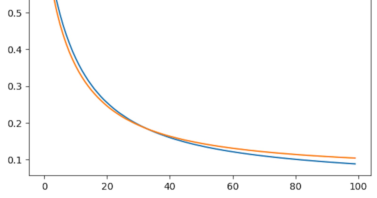
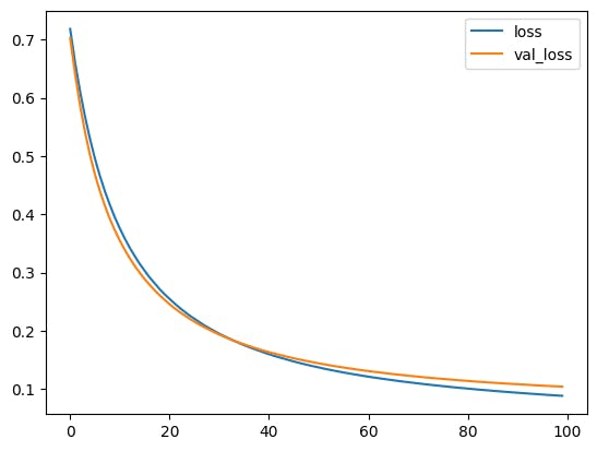
plt.plot(result.history['loss'], label='loss') # loss per epoch
plt.plot(result.history['val_loss'], label='val_loss') # validation loss per epoch
plt.legend()
Out:
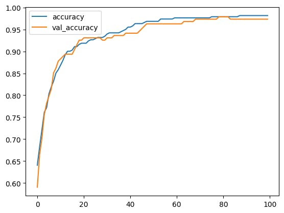
plt.plot(result.history['accuracy'], label='accuracy') # training accuracy per epoch
plt.plot(result.history['val_accuracy'], label='val_accuracy') # validation accuracy per epoch
plt.legend()
Out: