

We've completed the data preparation stage, where we have cleaned the data, processed it to get desired features, and understood the data to some extent.
Before we go into the initialization stage, we have one more step that can be considered part of data preparation. It is feature scaling or standardization. Although it's not always necessary, it is often a good idea to standardize the features to give them equal weight, especially when they are on different scales or units.
Each feature that has equal weight contributes equally to the distance measure. If one feature is in the range of thousands and another is in the range of tens, the feature with the larger scale could dominate when calculating distances. To prevent this differing magnitude of the features, features are often normalized or standardized, which ensures they are on a similar scale and contribute equally to the model.
Feature scaling is a method used to normalize the range of independent variables or features of data. In data processing, it is also known as data normalization. There are two common ways of performing feature scaling:
- Normalization has the effect of squeezing values into the range from 0 to 1. In cases where all input features need to be positive, this can be quite useful. But normalization does not handle outliers very well; if you have even one outlier that is much larger than the rest, all other values will appear to be very close to 0.
# x is the original value, min(x) is the smallest value in the dataset, and max(x) is the largest value.
# As a result of this operation, the smallest value becomes 0, the largest value becomes 1, and all other values will be scaled to fit within this range.
(x - min(x)) / (max(x) - min(x))
- Standardization is much less affected by outliers. It scales the data to have mean 0 and variance 1. The advantage of standardization is that it retains useful information about outliers and makes the algorithm less sensitive to them in contrast to normalization, which scales the data to a tight, specific range.
# x is the original value, mean(x) is the average of all values, and stdev(x) is the standard deviation.
# As a result of this operation, the average (mean) value will be scaled to 0, values one standard deviation above the mean will be scaled to 1, values one standard deviation below the mean will be scaled to -1, and all other values will be scaled based on how many standard deviations they are from the mean.
(x - mean(x)) / stdev(x)
We can decide to either standardize or apply a log transformation based on the distribution of the data. For instance, if the data is highly skewed (to the left or to the right deviating from the symmetrical bell curve), we might prefer to apply a log transformation.
However, these two methods are not mutually exclusive. It's common to apply a log transformation first to handle skewness, and then standardize the data. This is because the log transformation can reduce skewness and the impact of outliers, while standardization can scale the features to have a mean of 0 and a standard deviation of 1, which is often beneficial for machine learning algorithms.
We will reduce the skewness of the features and also bring the values closer together by applying these transformations to our data.
First, we're going to apply a logarithm transformation to reduce the skewness of the features. If you were to plot a histogram of your data, you'd see that data is skewed if the plot is not symmetrical and one side extends more than the other.
We're applying a log transformation to the Freq, SaleAmount, and ElapsedDays features. However, before we apply the log transformation, we need to make sure that these features do not contain any zero or negative values because the logarithm of zero or negative numbers is undefined. We'll need to convert ElapsedDays to a number of days. Right now, ElapsedDays is a date, and we're interested in the recency, which means how many days ago the last purchase was.
# Get the most recent purchase date
latest_purchase = max(customer_df['ElapsedDays'])

customer_df['ElapsedDays'] = (latest_purchase - customer_df['ElapsedDays']).dt.days
Then check the minimum values of these columns:
customer_df[['Freq', 'SaleAmount', 'ElapsedDays']].min()
Output:
Freq           1.00
SaleAmount     3.75
ElapsedDays    0.00
dtype: float64
If all the minimum values are greater than 0, you can proceed with the log transformation. If not, you'll need to adjust the values (e.g., by adding a small constant) so they're all positive before proceeding.
We have a minimum value of 0 in the ElapsedDays column and no value is less than 1 in the other 2 columns. So we can safely apply the log transformation by adding 1 to your values, which will turn all 0s into 1s (and the log of 1 is 0).
# Applying log transformation
import numpy as np

customer_df['Freq_log'] = np.log1p(customer_df['Freq']) # equivalent to np.log(customer_df['Freq'] + 1)
customer_df['SaleAmount_log'] = np.log1p(customer_df['SaleAmount'])
customer_df['ElapsedDays_log'] = np.log1p(customer_df['ElapsedDays'])
np.log1p()appliesnp.log(x+1)transformation. It's useful when especially x is very close to zero, because it handles x=0. It helps avoid underflow and loss of precision errors.
customer_df.head()
Out:
| CustomerID | Freq | SaleAmount | ElapsedDays | ElapsedDays_log | Freq_log | SaleAmount_log | |
| 0 | 12346 | 0.693147 | 11.253955 | 325 | 5.786897 | 0.526589 | 2.505849 |
| 1 | 12347 | 5.209486 | 8.368925 | 1 | 0.693147 | 1.826078 | 2.237398 |
| 2 | 12348 | 3.465736 | 7.494564 | 74 | 4.317488 | 1.496434 | 2.139426 |
| 3 | 12349 | 4.304065 | 7.472245 | 18 | 2.944439 | 1.668474 | 2.136796 |
| 4 | 12350 | 2.890372 | 5.815324 | 309 | 5.736572 | 1.358505 | 1.919174 |
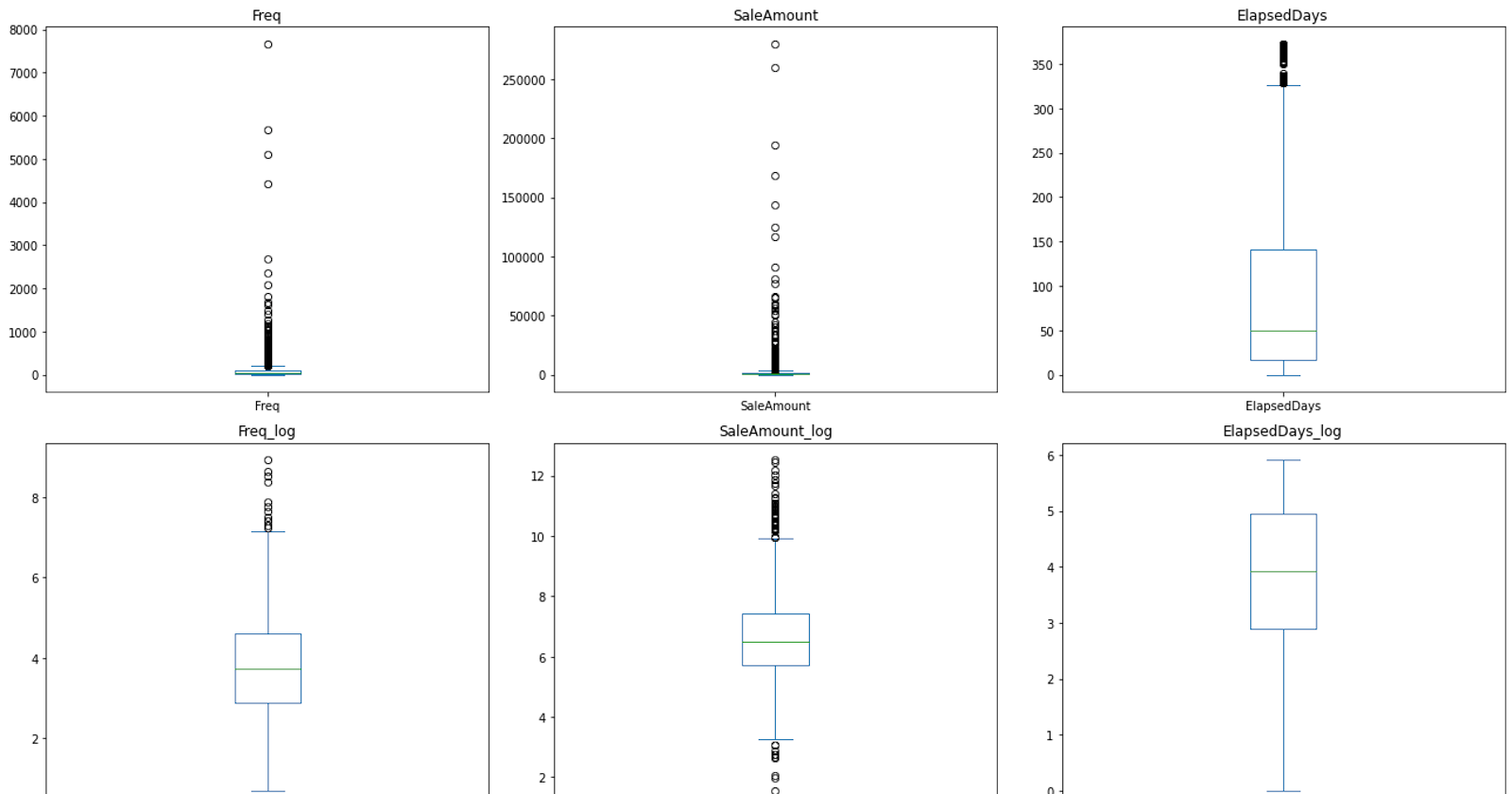
After the log transformation, the skewness of the data should be reduced. You can visualize this with histograms or box plots.
# Visualize the distribution
# Import the necessary library
import matplotlib.pyplot as plt

plt.figure(figsize=(18,10))

plt.subplot(2, 3, 1)
customer_df['Freq'].hist(bins=30)
plt.title('Freq')

plt.subplot(2, 3, 2)
customer_df['SaleAmount'].hist(bins=30)
plt.title('SaleAmount')

plt.subplot(2, 3, 3)
customer_df['ElapsedDays'].hist(bins=30)
plt.title('ElapsedDays')

plt.subplot(2, 3, 4)
customer_df['Freq_log'].hist(bins=30)
plt.title('Freq_log')

plt.subplot(2, 3, 5)
customer_df['SaleAmount_log'].hist(bins=30)
plt.title('SaleAmount_log')

plt.subplot(2, 3, 6)
customer_df['ElapsedDays_log'].hist(bins=30)
plt.title('ElapsedDays_log')

plt.tight_layout()
plt.show()
Out:
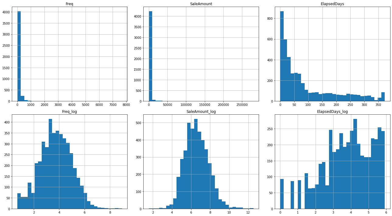
The asymmetry in the histogram can mean skewness of the distribution.
plt.figure(figsize=(18,10))

plt.subplot(2, 3, 1)
customer_df['Freq'].plot(kind='box')
plt.title('Freq')

plt.subplot(2, 3, 2)
customer_df['SaleAmount'].plot(kind='box')
plt.title('SaleAmount')

plt.subplot(2, 3, 3)
customer_df['ElapsedDays'].plot(kind='box')
plt.title('ElapsedDays')

plt.subplot(2, 3, 4)
customer_df['Freq_log'].plot(kind='box')
plt.title('Freq_log')

plt.subplot(2, 3, 5)
customer_df['SaleAmount_log'].plot(kind='box')
plt.title('SaleAmount_log')

plt.subplot(2, 3, 6)
customer_df['ElapsedDays_log'].plot(kind='box')
plt.title('ElapsedDays_log')

plt.tight_layout()
plt.show()
Out:
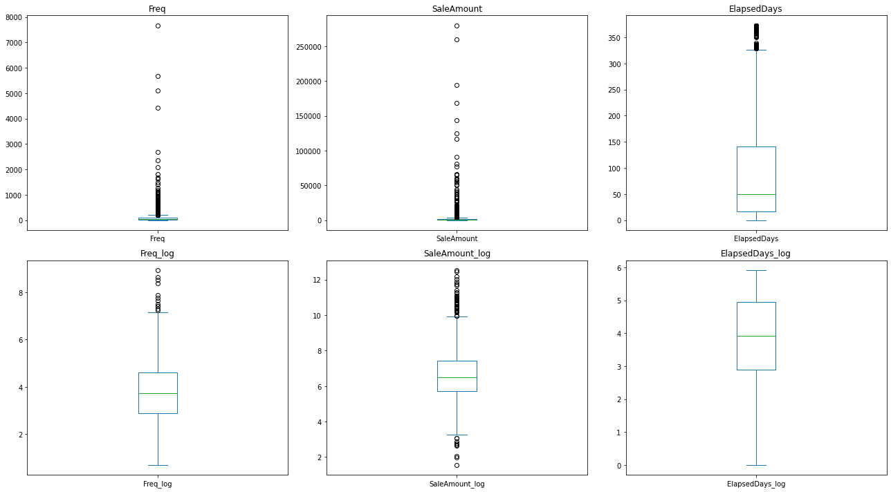
If the line in the box (the median) is not in the middle of the box, or the whiskers are not of equal length, it can suggest skewness.
For a quantitative measure of skewness instead of an impression of skewness, we calculate it with scipy.stats.skew().
from scipy.stats import skew

print("Skewness of Freq: ", skew(customer_df['Freq']))
print("Skewness of SaleAmount: ", skew(customer_df['SaleAmount']))
print("Skewness of ElapsedDays: ", skew(customer_df['ElapsedDays']))
print("Skewness of Freq_log: ", skew(customer_df['Freq_log']))
print("Skewness of SaleAmount_log: ", skew(customer_df['SaleAmount_log']))
print("Skewness of ElapsedDays_log: ", skew(customer_df['ElapsedDays_log']))
Out:
Skewness of Freq:  18.037289818570194
Skewness of SaleAmount:  19.332680144099353
Skewness of ElapsedDays:  1.2456166142880103
Skewness of Freq_log:  -0.01230439000937588
Skewness of SaleAmount_log:  0.3964614244871878
Skewness of ElapsedDays_log:  -0.5543745693187032
Finally, we're going to standardize log-transformed features. Standardization transforms the data to have a mean of 0 and a standard deviation of 1. This helps ensure that all features have equal weight when applying machine learning algorithms.
from sklearn.preprocessing import StandardScaler

# Initialize a scaler
scaler = StandardScaler()

# Set up the X_features
X_features = customer_df[['Freq_log', 'SaleAmount_log', 'ElapsedDays_log']]

# Fit the scaler to the log transformed features and transform
X_features = scaler.fit_transform(X_features)

# Save the scaled features
scaled_df = pd.DataFrame(X_features, columns=['Freq_scaled', 'SaleAmount_scaled', 'ElapsedDays_scaled'])
customer_df = pd.concat([customer_df, scaled_df], axis=1)

customer_df.columns
Out:
Index(['CustomerID', 'Freq', 'SaleAmount', 'ElapsedDays', 'Freq_log',
       'SaleAmount_log', 'ElapsedDays_log', 'Freq_scaled', 'SaleAmount_scaled',
       'ElapsedDays_scaled', 'Freq_scaled', 'SaleAmount_scaled',
       'ElapsedDays_scaled'],
      dtype='object')
Now, the data is ready for the k-means clustering algorithm.